

Content
History
In late march 2023 llama.cpp really took off, it was trending on hackernews due to a misunderstanding of a new mmap feature
[1]. Where the authors thought they found some "sparsity" property of the Transformer, but turned out to just be a quirk of how the OS shows memory usage with mmap.
Some notable developments:
- .ggml is depricated in favor of .gguf to avoid breaking backwards compatibility when new values are added.
- Metal support was added in June 2023 (https://github.com/ggml-org/llama.cpp/pull/1642)
- Chat-templates supporting Jinja templates is supported. This took some time due to llama.cpp s focus on simplicity. Luckily Google released Minja which is a minimal Jinja parser with the only goal of supporting all LLM chat-templates.
Some notable contributors key to the success of llama.cpp:
- Georgi Gerganov (GG), the full-scope mastermind behind the GGML project.
- TheBloke's work with publishing quantized models on HF blazingly fast.
- Kawrakov for quantization research and optimization. Now left for his own fork ik_llama.cpp.
- Jart/Slaren for the
mmapfeature and much more. - And many more...
Overview
In this guide we focus on the less talked about parts, step 3 and 4 in the figure below. Which is really pure GGML functionality and is mostly concerned with how llama_context::decode_μbatch is implemented.
We will focus on how the computational graph is built, how it is executed on backend(s), and how the kv cache is updated.
In the future I might make a post on how the different kinds of sampling strategies works when calling select_next_token(output) with output being an 1d tensor of length $|V|$ representing a distribution over the vocabulary $V$. Also how llama.cpp handles more complex strategies like beam-search that relies heavily on the kv cache. Another interesting part is how a context-free-grammar can be applied to generate
# 1: Parse .GGUF format and load/mmap weights
model = load_model_weights("model.gguf")
# 2: Tokenize the prompt/context
context_tokens = tokenize(prompt_text)
while not generation_complete(context_tokens):
    # 3: Build computational graph of model and set inputs
    cgraph = build_computational_graph(model)
    cgraph.set_inputs(context_tokens, kv_cache)
    # 4: Execute graph on backend(s)
    output = execute_graph(cgraph)
    # 5: Select next token from output
    next_token = select_next_token(output)
    context_tokens.append(next_token)
Some important flags to be aware of for llama_cli are:
-n MAX_GEN, sets the maximum number of calls todecode_ubatch, (first PP can hold multiple tokens) so totally processed tokens will ben_prompt+MAX_GEN-1. This is useful to limit the number of tokens generated.-c Nor--ctx-size Nsets the actual context length toN. Which determines KV cache size etc. (KV cache is set to a rounded up to power of 2 of context length)--no-warmupdisabling the warmup PP step which is annoying when debugging.
A note about the relations between GGML and llama.cpp:
GGML and llama.cpp are developed simultaneously, and llama.cpp can be compiled with a system GGML library by setting the LLAMA_USE_SYSTEM_GGML cmake flag, or with the included GGML source. Georgi takes care of the two-way syncing using scripts/ggml-sync.sh.
The ggml_tensor
Akin to all ML libraries and frameworks, the Tensor object is the core part of it. All operations are performed on tensors and all types of data are tensors. In comparison to its mathemtical counterpart, ML Tensors are more than just a multi-linear transformation, as evident below:
// Simplified version of ggml_tensor
struct ggml_tensor {
  enum ggml_type type; // Data type e.g., f16, q4_0, q4_K
  enum ggml_op op; // which operator e.g., addition/relu

  int64_t ne[GGML_MAX_DIMS]; // number of elements
  size_t  nb[GGML_MAX_DIMS]; // stride in bytes:
  // nb[0] = ggml_type_size(type)
  // nb[1] = nb[0]   * (ne[0] / ggml_blck_size(type)) + padding
  // nb[i] = nb[i-1] * ne[i-1]

  int32_t op_params[GGML_MAX_OP_PARAMS]; // Parameters for the operator
  struct ggml_tensor * src[GGML_MAX_SRC]; // source tensors
  struct ggml_backend_buffer * buffer; // which backend
  void * data; // The actual pointer to the data
};
In ggml.c/llama.cpp every tensor is represented by a 4 dimension tensor, which makes sense since we want the struct to be as small as possible with static size arrays. Four is a reasonable choise since more than 4d tensors are very rare in the LLM space, 4d tensors are common though, as the self-attention layer contains $Q,K,V\in\mathbb{R}^{B\times h\times d\times L}$ for example. Its shape is stored in reverse order from what you typically expect in torch for example, so a 3d tensor $(d_1, d_2, d_3)$ would be $(d_3, d_2, d_1, 1)$.
A ggml_tensor is really more than just a tensor, it's more like a node in a computational graph, just like in other autodiff libraries like torch, since it includes sources and operations. We can of-course still represent leaf nodes like weights using ggml_type.GGML_OP_NONE.
At a lower level a tensor (in computer science) is defined as a composition of a Layout (shape and stride) and a data engine (pointer to data). To be fast this is really what metal/CUDA kernels operate on.
A $(4, 2)$ matrix in f32 (4 bytes/cell) has shape $(2, 4, 1, 1)$ and stride $(4, 8, 32, 32)$ moving along a row is +4 bytes for each cell, and if we want to move down we have to skip the whole row which is +8 bytes.
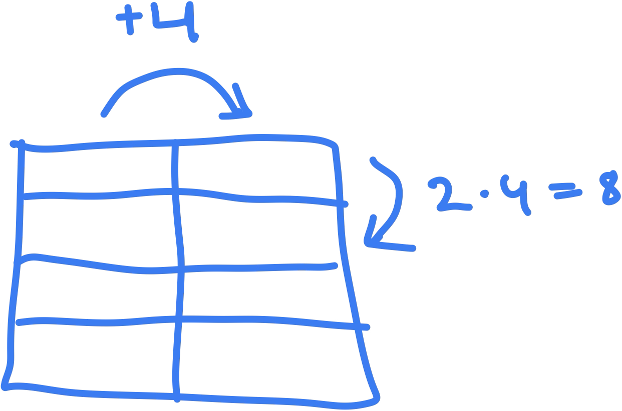
This is one of the fundamental concepts for memory layouts and is key to CUTLASS CuTe Layout, which can further be extended to handle different tilings in a unified way, heavily used in CUDA kernels.
The Computational Graph (ggml_cgraph)
The ggml_tensor allows for a simple way to build a graph, since the tensors are the nodes.
The final result tensor is already representing the full computational graph. ggml_cgraph just makes an explicit ordering in a list as seen in the definition below:
struct ggml_cgraph {
  int n_nodes; // number of nodes currently in use
  int n_leafs; // number of leafs currently in use
  struct ggml_tensor ** nodes; // tensors with data that can change if the graph is evaluated
  struct ggml_tensor ** leafs; // tensors with constant data
  struct ggml_hash_set visited_hash_set; // Used during traversal so we don't add duplicates
  enum ggml_cgraph_eval_order order;     // Order which source nodes are visited.
};
Here we construct a simple model of $A^T(AB)$ in pure ggml.c.
ggml_context* ctx = ggml_init(params);
ggml_tensor* a    = ggml_new_tensor_2d(ctx, GGML_TYPE_F32, cols_A, rows_A);
ggml_tensor* b    = ggml_new_tensor_2d(ctx, GGML_TYPE_F32, cols_B, rows_B);
// memcpy data into a,b or point data in a,b to already existing data if ctx->no_alloc is set
ggml_cgraph* gf   = ggml_new_graph(ctx);
ggml_tensor* result;

result = ggml_mul_mat(ctx, a, b);
struct ggml_tensor* at = ggml_transpose(ctx, a);
at = ggml_cont(ctx, at);
result = ggml_mul_mat(ctx, at, result);

// Traverse the graph and add the nodes to gf
ggml_build_forward_expand(gf, result);
ggml_graph_dump_dot(gf, NULL, "llama.dot"); // Visualize the graph
// do computation with graph and then free memory with ggml_free(ctx);
Once we create the graph we visualize it as seen in the figure below.
Once ggml_build_forward_expand(graph, node) is called, the graph is traversed from node in recursive fashion until leaf nodes are reached. Creating a list of topological sorted nodes in ggml_cgraph.nodes.
Every node is an operator like ggml_add, ggml_mul_mat, ggml_relu etc., which has an array of source nodes. So no operations are done until the cgraph is actually executed. Hence, in the code above no computation has been done.
The ggml_context is nice because it has the collection of all the tensors and the graph, so when we want to free
all the tensors we simply call ggml_free(ctx).
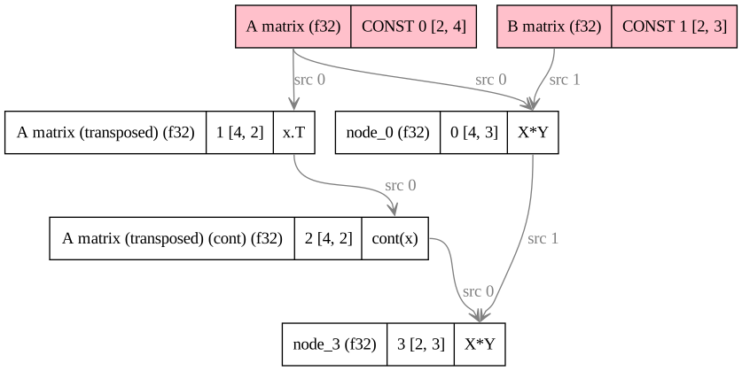
ggml_graph_dump_dot() for graph representing $A^T(AB)$. Red nodes are leaf nodes (essentially the inputs to the graph), in this case matrix $A$ and $B$. After a forward pass, node_3 the root node, holds the result. Note that ggml_mul_mat expects a contiguous memory layout for its inputs, hence we have to make the transposed matrix contiguous using ggml_cont.
The llm_graph_context
The llm_graph_context is the base class of all LLM implementations, just as we did above in the toy example, we define the LLM's architecture in terms of a GGML computation graph. Most LLMs are Transformers, so there's already many helper function available for rope, attention, feed-forward etc., making it easier to implement the layers of self-attention and feed-forward operations. And whenever a new architecture comes along, we have to define its computational graph here. For example to add GPT-OSS we need to think about the sink softmax. And if we think the operation is fundamental and generic enough we might even add it to GGML and create optimized kernels for it.
llama_model.cpp.
Execution
In the llama_context::llama_context constructor we set the available backends in the array llama_context::sched.backends.
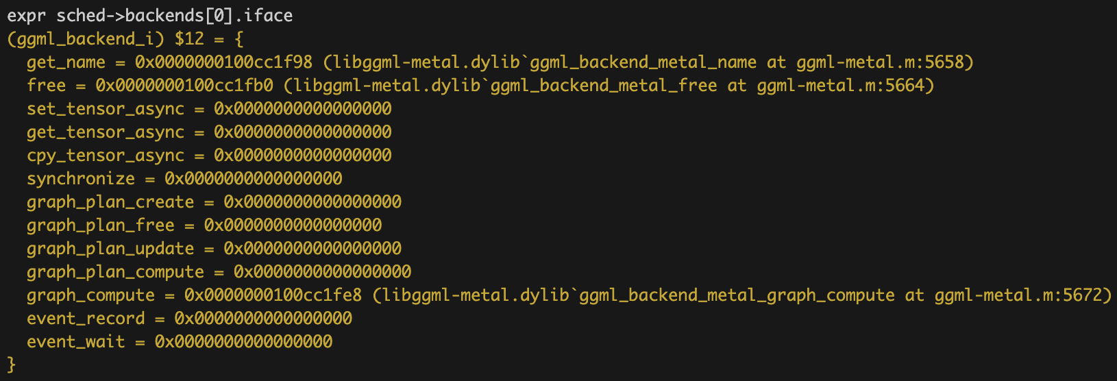
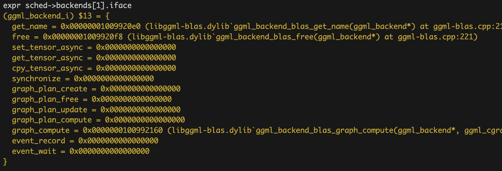
In my case on a MacBook M4, we have three backends available by default: cpu, blas and metal. The figure below shows how each backend implements a graph_compute function, etc.
graph_compute etc.
When we later do the compute, we pass the available backends:
ggml_backend_sched_graph_compute_async(sched.get(), gf);
This triggers the scheduler to partition the computation graph across backends. The scheduler walks through the graph and assigns each operation to the most suitable backend based on if the backend implements the operation, which device the tensor currently resides and more. The actual computation happens in ggml_backend_sched_compute_splits:
static enum ggml_status ggml_backend_sched_compute_splits(ggml_backend_sched_t sched) {
    // Each split represents a contiguous subgraph assigned to one backend
    for (int i = 0; i < sched->n_splits; i++) {
        struct ggml_backend_sched_split * split = &sched->splits[i];
        ggml_backend_graph_compute(split->backend, split->graph);
    }
}
To bridge metal kernel execution there are three alternatives swift, objc, and c++, and llama.cpp uses objc and is implemented in ggml-metal.m.
The Metal backend
The main job of ggml_metal_graph_compute() is to keep the GPU busy, so it must encode kernels quickly to the command buffers. Main thread starts with first 128 nodes, then uses 1-2 threads to do encode them. Gaps between kernels are simply a waste since the GPU is idle.
Metal kernels are executed sequentially, so simple encoding the command buffers in the topological ordering of the ggml_cgraph.nodes is enough. We just have to make sure different threads work in order and uses commandBuffer waitUntilCompleted to wait for the previous kernels to finish.
Metal kernels are have a slighly convoluted setup, with many types of queues, buffers, encoders, etc. Here is an overview of the steps:
-
To dispatch a kernel to the selected device (e.g. the GPU given by
MTLCreateSystemDefaultDevice()) we create a command queue ([device newCommandQueue]). -
Next, we set up the buffers for the input and output data (
[device newBufferWithLength:options:]), since memory is shared between device and host we don't have to copy any memory. -
Next the pipeline state has to be created that contains a reference to the kernel function.
-
We create a compute command encoder which sets the pipeline state and binds the buffers.
-
We specify the dispatch thread strategy using
dispatchThreadgroups:threadsPerThreadgroup -
Commit the command buffer to the GPU using
commandBuffer commit, which hands over the control to the GPU, which will execute it as soon as possible. -
This is asynchronous, so we have to wait for the kernel to finish using
commandBuffer waitUntilCompleted.
Step 2 here differs from CUDA significantly as it must copy the data:
cudaMemcpyAsync((char*)tensor->data+offset, data, size, cudaMemcpyHostToDevice, cuda_ctx->stream())
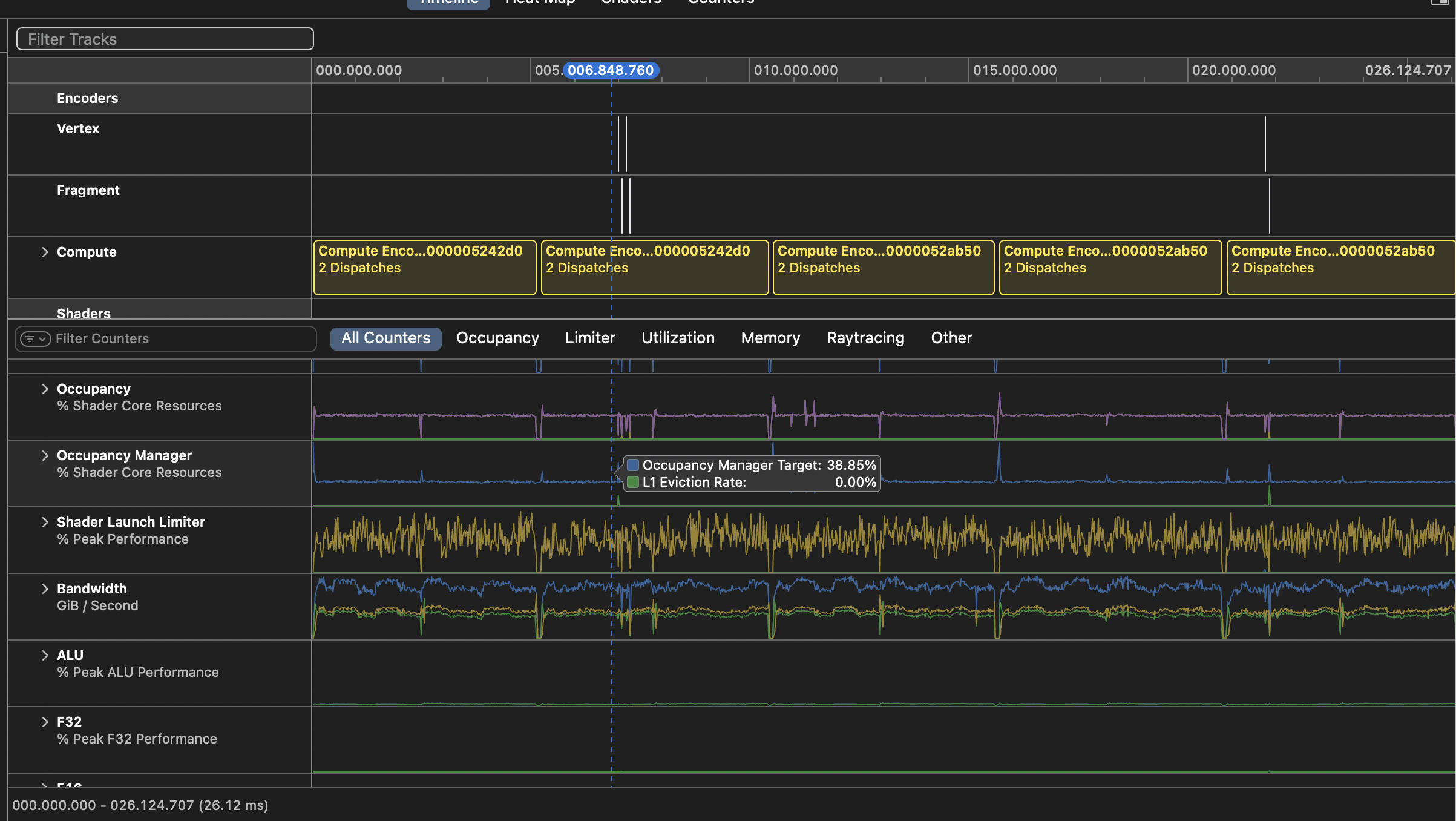
We can also profile and debug by capture traces of the kernels using MTLCaptureManager and by setting the MTL_CAPTURE_ENABLED=1 environment variable the trace is saved to /tmp/perf-metal.gputrace which we then can open with Xcode. Below is a simple trace that I ran executing 5 matmuls after eachother.
Kernels
What an overloaded term... Anyways, how are quantized matmuls done?
Quantized matmul
In the forward pass of a quantized model, let's go with Q4_K in this case, multiple types of matrix multiplcations are used. For optimization depending on the dimensions, either matrix vector multiplcations are dispatched, or full matrix-matrix kernels.
At a high level we can think of the hidden state passing through the transformer, this is kept in f16 or f32, while the weight matrices are quantized. Hence, we have multiple types of matmuls where the types differ from src0 and src1. Since the KV cache is kept in f16 by default we also get matmuls with Q4_K and f16, f16 and f32, etc. Those uses kernels such as GGML_METAL_KERNEL_TYPE_MUL_MV_EXT_Q4_K_F32_R1_5 and GGML_METAL_KERNEL_TYPE_MUL_MM_F16_F32.
llama.cpp handles the many combinations of type pairs neatly, using templated kernels as shown below, even allowing function pointers handy for the dequantization step.
template<
  typename T,
  typename T4x4,
  typename simdgroup_T8x8,
  typename block_q,
  short nl,
  void (*dequantize_func)(device const block_q *, short, thread T4x4 &)
> kernel void kernel_mul_mm(...);
In future blog posts we will take a look at the actual implementations and see how threadgroup memory is used in similar fashion how cuda kernels use SMEM.
Sink softmax
Here is the PR where the sink softmax was added: https://github.com/ggml-org/llama.cpp/pull/15091/
MoE matmuls
To support MoE each matmul kernel also has an "indexed" or "indirect" variant, which also takes in a tokens per expert (tpe) parameter.
Flash-attention in Metal
llama.cpp has support Flash-attention for many quantization formats, e.g. GGML_METAL_KERNEL_TYPE_FLASH_ATTN_EXT_Q4_0_H64 with an intricate dispatch strategy depending on dimensions. Luckily we can generate Flash-attention kernels for specific attention shapes, with Turner's impressive write-up:
https://github.com/philipturner/metal-flash-attention
mmap and Memory Management
One important thing is tensors are not loaded individually, but as one contiguous memory region. Then offsets determine where each tensor starts. The tensors' metadata is then iterated over and depending on the type of weight the backend is set, for example the input layer could always be on cpu, while the rest is on metal.
So some backends support pointing to mmap'd memory, basically only SoC and cpu. For example discrete GPUs like cuda does not support this since the memory space is separated, although it could potentially work for a Jetson SoC.
The code goes something like this when setting the buffer buf for each backend the tensors from file:
// Create backend buffer that directly references mmap'd memory
if (use_mmap && backend in ["BLAS", "Metal", "CPU"]) {
  ggml_backend_buffer_t buf = ggml_backend_dev_buffer_from_host_ptr(
      dev,
      (char *) addr + first,  // mmap'd file region
      last - first,           // size
      max_size
  );
} else {
  // Copy from mmap'd memory to backend buffer
  ggml_backend_buffer_t buf = ggml_backend_alloc_ctx_tensors_from_buft(ctx, buft);
}
So we now understand how the weights are loaded and mmaped on to the backend buffers. Each backend has its context which will contain all tensors that it's referencing. But these are only the weight tensors, the later to be leafs in the computation graph. The computation graph contains both these leafs and all the other intermediate nodes that must be allocated. How does this play together? Basically the graph contains nodes that are already mmaped, and nodes that yet have no data pointer.
When ggml_gallocr_alloc_graph() runs, it checks if the data pointers is set for each node, if not it will set it.
Note here that it's important to distinguish between actually allocating memory and setting the data pointer. Setting the data pointer is refered to as initializing the tensor.
Why not run a metal kernel on iOS or your TV?
Well, lots of devices run Apple Silicon, and it turns out we can run Metal kernels on iOS devices, ipadOS, watchOS and tvOS. They are just slower focusing more on efficiency cores.
With XCFramework we can compile a library for all those platforms and use llama.cpp on your iPhone etc.
What about vLLM and SGLang?
Inference frameworks fall into two categories, single user and multi user. llama.cpp being a single user focused, i.e., for the individual user to run on their own device and hence must be very portable. While vLLM and SGLang are multi user focused, i.e., more business focused and therefor optimises for modern top GPUs and so on.
The multi-use focus of these frameworks is evident in their great support for continuous batching, custom attention algorithms and caching. See vLLM's PagedAttention and SGLang's RadixAttention with prefix caching. Also their DSL is interesting.